The Sun is a variable star and the amount of energy it emits varies from month to month, year to year, and century to century. One of the manifestations of these variations are sunspots, which are more common when the Sun is more active and disappear when it is less active. These spots follow a solar cycle of about 11 years, but sometimes there is a longer period, decades or centuries, when the Sun’s activity is so low that there are no spots. These periods are called grand solar minima. There are also periods of decades or centuries when the activity is higher. These are called grand solar maxima.
The Sun provides 99.9% of the energy that the climate system receives. So, there have always been scientists who thought that variations in the Sun were the cause of climate change. The problem is that they never had enough evidence to prove it. Until now.
The IPCC and NASA say…
The IPCC and NASA are convinced that changes in the Sun have very little effect on climate. They rely on two arguments. The first is that changes in solar activity are very small. We measure them with satellites because they cannot be measured from the surface, and we know that the radiant energy coming from the Sun varies by only 0.1%. The magnitude of the changes is better appreciated when we use the full scale. Many scientists believe that such a small change can only produce small changes in climate.
The second argument is that the evolution of temperature does not coincide with the evolution of solar activity. Since the 1990s, solar activity has decreased while warming has continued.[i]
Actually, this argument is not valid because it does not say that the Sun does not affect temperature, but that it is not the only factor in doing so, something we already knew because temperature responds to many factors such as El Niño, volcanoes, the polar vortex, or changes in the Earth’s orbit. There are many natural causes that change the climate, and what we need to know is whether the Sun is one of the main ones.
To find out, we don’t need to care what the IPCC and NASA think, we need to ask the climate itself. It doesn’t matter how small the changes in the Sun are if it turns out that the climate responds strongly to them by causing big changes.
Climate during the Holocene
And the best way to find out is to look at what has happened to the climate over the last 11,000 years, the interglacial period we call the Holocene. The advantage of doing this is that the Holocene climate changes could not have been caused by changes in CO₂. They must have been caused by something else.
To study the climate of the past, scientists use various climate proxies that they collect in different parts of the world. A major study published in Science used 73 of these proxies to reconstruct Holocene climate.[ii] I have used the same proxies, with a slight modification in the way they are mixed.
What we see, and what a large number of studies also support, is that there was a warm period of thousands of years, called the Climate Optimum, followed by a long period of cooling, called Neoglaciation.
How do we know that this reconstruction is correct? Another study reconstructed the progress of the Earth’s glaciers over the past 11,000 years.[iii] They divided the globe into 17 regions, and this graph shows the number of regions whose glaciers increased in size during each century of the Holocene.
Since glaciers grow when it is colder, we can invert their figure and compare it to the temperature reconstruction graph so that its meaning is the same. We find a high degree of agreement. The glaciers confirm what the temperature reconstruction shows. We also know that CO₂ has done the opposite of temperature, but that is a story for another day.
Note: y-axis is the Z factor, which is related to temperature anomaly.
Both graphs also show some severe cooling episodes that were accompanied by increased glacier growth. These abrupt climate events of the past have been studied and identified by paleoclimatologists. Of all of them, we will focus on four of the most important ones. The Boreal Oscillation, the 5.2 kiloyear event, the 2.8 kiloyear event, and the Little Ice Age.
The four are separated by multiples of 2,500 years and form a cycle that I have called the Bray cycle because that was the name of the scientist who discovered it in 1968.[iv]
Now that we know the climate of the past, we need to talk about the activity of the Sun in the past.
Past solar activity
The Sun’s activity is recorded in the tree rings through the action of cosmic rays. A constant stream of cosmic rays from the galaxy reaches the solar system. Some interact with the atmosphere. Some collide with nitrogen in the atmosphere, converting it to carbon-14, which is heavier than normal carbon-12 and radioactive. This carbon-14 combines with oxygen to form radioactive CO₂, which is breathed by trees. The carbon is used in photosynthesis to make cellulose, which allows the tree trunk to grow in diameter. When the tree dies, the carbon-14 in the wood slowly decays over centuries and millennia. You just have to measure how much carbon-14 is left in the wood to know how much time has passed since the tree died.
Each growth ring of a tree records the carbon-14 that was in the atmosphere that year, and scientists have used millennia-old trees and preserved logs to construct a calibration curve that spans tens of thousands of years. This allows them to determine the age of any organic remains, even if it is not a tree trunk, just by knowing the carbon-14 it contains. This is known as radiocarbon dating.
The only problem is that the production of carbon-14 by cosmic rays is not constant. The Sun’s magnetic field deflects the path of cosmic rays, causing many to miss the Earth, and changes in the Sun’s activity affect its magnetic field.
As the Sun’s activity increases, fewer cosmic rays arrive, less carbon-14 is produced, and organic remains appear older because they contain less of it. When the Sun’s activity becomes weaker, more cosmic rays arrive, more carbon-14 is produced, and the organic remains look younger because they contain more of it.
This produces deviations in the calibration curve that allow us to know what the Sun’s activity was in the past.
Spörer-type solar minima
When we analyze the radiocarbon curve over the last 11,000 years, we observe large deviations that indicate long periods of low solar activity. These extended periods of low solar activity are called grand solar minima and increase carbon-14 production by 2%. The most common ones last about 75 years, and there have been about twenty in the last 11,000 years. The most recent was the Maunder Minimum in the late 17th century. But there are other types of grand solar minima that are much more severe because they last twice as long, about 150 years. The last of these severe solar minima was the Spörer Minimum, which occurred in the 15th and 16th centuries.
There have been only four such Spörer-type grand minima in the entire Holocene. 2,800 years ago, there was the Homer Minimum, 5,200 years ago the Sumerian Minimum, and 10,300 years ago the Boreal Minimum. We know when they occurred thanks to tree rings.
If the dates sound familiar, it is because the four grand Spörer-type Holocene minima coincide exactly with the four major climatic events on the graph we saw earlier. We know that during each of these grand solar minima, when the Sun’s activity dropped for 150 years, the climate experienced a tremendous cooling that had a major effect on climate proxies around the globe.
We also know that low solar activity during the grand minima has had a major impact on human populations. Past human settlements and their component structures can be radiocarbon dated. When humans were doing well in the past, the population grew and they built more, and when they were doing poorly, usually because there was less food, the population decreased and they built less. Scientists have estimated the evolution of the human population of the British Isles by analyzing the radiocarbon dates of thousands and thousands of remains from hundreds of archaeological excavations.[v]
What they have found is that the population increased greatly with the advent of agriculture, but every time there was a severe deterioration in the climate, the human population suffered from diminishing resources. And the largest declines occurred when grand Spörer-type solar minima took place. Other population declines also coincide with other cooling periods, confirming our reconstruction.
This tells us that the worst climate changes in the past have been caused by changes in solar activity. It also tells us that what is bad for humanity is cooling, not warming.
Now we can respond to the IPCC and NASA. Never mind that solar irradiance changes very little, and never mind that temperature does not always do the same thing as solar activity. Clearly there are other factors at play. But we can state emphatically that changes in solar activity affect the climate because that is what the climate says. The study of past climate leaves no room for doubt. The Sun changes the climate. And if we don’t know how it does it, we should study it.
The 20th century solar maximum
Since low solar activity causes cooling, it stands to reason that high activity must cause warming. Solar activity in the 20th century was very high, in the top 10% of the last 11,000 years.
If we count the number of sunspots in each solar cycle over the last 300 years and divide by the length of each cycle, we can see how much solar activity has deviated from the average. Since the Maunder Minimum, during the Little Ice Age, solar activity has been increasing and was well above average between 1933 and 1996, a period of six cycles of increased solar activity that formed the 20th century solar maximum.
Although we cannot know how much of the 20th century warming is due to this modern solar maximum, there is no denying that it is a significant part, because as we have seen, the Sun has been the cause of much of the major climate change over the past 11,000 years.
Conclusions
There are two pieces of good news. The first is that solar activity cannot rise above the 20th century maximum. It is not like CO₂, which can keep going up. The Sun’s activity can stay high or go down, but it cannot go up, so the warming should not accelerate and should not be dangerous.
In 2016, I developed a model to predict solar activity in the 21st century. At the time, some scientists believed that solar activity would continue to decline until a new grand solar minimum and mini-ice age. But my model predicts that solar activity in the 21st century will be similar to that of the 20th century. It also predicted that the current solar cycle, the 25th, would have more activity than the previous one, and it was right.
The second piece of good news is that if much of the 20th century warming is due to the Sun, then there is no climate emergency. Believing that all climate change is due to our emissions is one of those errors that sometimes occur in science, like believing that the Earth is the center of the solar system, that interplanetary space is full of ether, or that stomach ulcers are caused by stress, not bacteria.
Where are the tears? Elephant Seals and Penguins were forced off the Ross sea 1,000 years ago because it got too cold
One thousand years ago Southern Elephant Seals were happily living in the Ross Sea of Antarctica. Likewise Adelie Penguins frolicked in the sun there during the “Penguin Optimum” of three to four thousand years ago. They had lived there on and off for thousands of years in the Holocene, but the glaciers came back and the cold times returned, and all the colonies were wiped out. All that’s left there now is just their rotting bones and fur as testament to the devastation of Global Cooling.
The Ross Sea is a part of Antarctica that is south of New Zealand, and in the pictures below the remains of the seals and penguins show that they had well established colonies in places where they are unable to live now. The red circles mark the seal colonies, and the blue stars show the penguins. The colonies ebbed and flowed but then were lost as the Little Ice Age began and have not recovered.
Today the beaches are an empty wasteland:
Today, the beaches are largely free of marine mammals and birds; skuas (Stercorarius maccormicki) are the most widespread species. Along the southern coast, penguins are absent, although small Adélie (Pygoscelis adeliae) rookeries existed in the past (i.e., Baroni and Orombelli, 1991, 1994a; Emslie et al., 2007). Adélies also occur adjacent to Terra Nova Bay at Adélie Cove and Inexpressible Island. Solitary or small groups of Weddell seals (Leptonychotes weddellii) occasionally haul out on the VLC. No other seals use these beaches at present.
The seals and penguins of Antarctica must be desperately hoping for some global warming so they can return to their ancestral homes and flourish where only desolate ice grips the sea and shore now. If only humans could do something about that!
Indeed, it’s time to launch a new campaign: “Fossil fuels can save the seals”. (It has just as much scientific validity as any eco-campaign running today, ask the IPCC!).
I don’t believe human emissions can warm the planet enough for the penguins to notice, but what if I’m wrong?
There really was a “Penguin Optimum” at about the same time as the Minoans and the Myceneans thrived. Bring back the warmth!
The red and yellow bars mark warmer eras where the marine mammals flourished. The diatom results marked in blue at the bottom (F. curta) of the graph below, show how sea ice expanded in the last thousand years as the cold made life impossible for the seals and penguins. The diatom results marked in red (T. antarctica) rise in the eras of longer warmer summers. The graph above runs “backwards” in time from right (the past) to left (present).
Tell the children, the world was warmer a thousand years ago, and the cooling has been a killer. If they like life on Earth, they want more warming, not more cooling. The world has been cooling for 5,000 years, and if we could warm the Earth that would be a good thing.
More evidence emerges that Antarctica has undergone rapid glacier and sea ice expansion in recent centuries, in line with the long-term and recent Antarctic cooling trend.
West Antarctica’s mean annual surface temperatures cooled by more than -1.8°C (-0.93°C per decade) from 1999-2018 (Zhang et al., 2023).
Not just West Antarctica, but most of the continent also has cooled by more than 1°C in the 21st century. See, for example, the ~1°C per decade cooling trend for East Antarctica (2000 to 2018) shown in Fig. ES1 (right).
According to a new study, about 6000 years ago Antarctica’s Collins Glacier’s frontline was a full 1 km southwest of its current extent. The frontline advanced to today’s extent ~5000 years ago.
“Previous studies proposed that 6000 yr BP, the frontline position of the Collins Glacier was located 1 km further south west than the present, and that the current frontline was first attained at approximately 5000 yr BP.”
The glacier then continuously retreated south of the modern extent for another 4000 years, with peak ice loss 1000 years ago (as shown in the 1000-year “Proglacial lake environment” image). In the last 1000 years this glacier has rapidly re-advanced back to the glaciated extent from 5000 years ago, which is in line with the sustained cooling trend ongoing since the Medieval Warm Period.
Throughout the Holocene (Medieval Warm Period, Roman Warm Period, and earlier) and until a few hundred years ago (from ~7100 to 500 years before present), coastal Antarctica’s Victoria Land (VLC) was substantially warmer than today. The Ross Sea was also sufficiently ice-free to allow for elephant seal populations (as large as ~200,000 individuals) to thrive at 73-78°S.
Today, however, elephant seal populations – which require extended sea ice-free sea waters to breed, forage, and provide nourishment for their pups – can no longer subsist anywhere even remotely close to the coasts of the Antarctic continent. It is now too cold and the sea ice is too extensive.
The substantially reduced number of remaining elephant seals existing today can only survive on subantarctic islands (South Georgia, Macquarie) at southern South American latitudes (~54.5°S) situated 2400 kilometers north of VLC (Koch et al., 2019).
The “genetically distinct” VLC elephant seal populations that endured throughout the Holocene and even through Medieval times have tragically died off in the last few centuries due to the modern-era cooling gradient and subsequent ice cover expansion (Hall et al., 2023).
“Across all sites, there is a precipitous drop in the number and geographic extent of the SES [southern elephant seals] remains within the last millennium”
“…the documented population crash and abandonment of the entire coast by SES after ~1000-500 yr BP was due to return of heavy sea ice”
And with the modern sea surface temperatures cooling and southern hemisphere sea ice expansion in recent decades, even the subantarctic islands in the South Pacific that SES are limited to occupying today may not be sufficiently warm and ice-free to accommodate remaining populations. Today’s southern elephant seals are thus ironically threatened by cooling in the era of anthropogenic global warming.
“[P]ack-ice expansion (both duration and extent) in the Ross Sea over the last several decades has been linked to reduced female foraging in this region, consequent low weaning weights and survival of pups, and ultimately the decline of the Macquarie Island population.”
Interestingly, Hall et al. also report that not only have the last few centuries (including the present) been “the coldest, iciest conditions in the post-glacial period” (see the blue sea ice and red temperature trend lines on the Holocene timeline), but even the last glacial period had periods (~50,000 to 25,000 years ago) with less sea ice than today, allowing SES to occupy the VLC coast.
Many viewers of Climate: The Movie have asked for more information on the topics discussed. In response, I selected the following 70 key statements from the movie and provide references and context for the statements here. Sometimes the statements are slightly paraphrased from what was said for brevity. The statements are listed in the same order as they appear in the movie. The references, illustrations, and links below are my attempt to clarify the statements, provide context, and support the idea behind the phrase or sentence.
I received help from Dr. Willie Soon and Marty Cornell in building this bibliography. My thanks to both.
These “27 estimates are a thin basis for drawing definitive conclusions about the total welfare impacts of climate change. Moreover, the 11 estimates for warming of 2.5 C indicate that researchers disagree on the sign of the net impact: 3 estimates are positive and 8 are negative. Thus it is unclear whether climate change will lead to a net welfare gain or loss.”Tol, 2018
Lomborg, B. (2020, July). Welfare in the 21st century: Increasing development, reducing inequality, the impact of climate change, and the cost of climate policies,. Technological Forecasting and Social Change, 156. doi:10.1016/j.techfore.2020.119981
Tol, R. (2023). Costs and benefits of the Paris Climate Targets. Climate Change Economics, 14(4). doi:10.1142/S2010007823400031
Tol, R. S. (2018). The Economic Impacts of Climate Change. Review of Environmental Economics and Policy, 12(1), 4-25. doi:10.1093/reep/rex027
Skepticism is career suicide and might be criminalized.
Unsettled, What Climate Science tells us, what it doesn’t, and why it matters, by Steven Koonin.
Climate proxies
A good overview of climate proxies:
Patalano, R., & Roberts, P. (2021). Climate proxies. In D. T. Potts, & E. Harkness, The Encyclopedia of Ancient History. John Wiley & Sons. doi:10.1002/9781119399919.eahaa00609
For a discussion of many of the best global temperature proxies that cover the past 12,000 years see Climate Catastrophe! Science or Science Fiction?, 2018, pp. 95-107.
May, A. (2018). Climate Catastrophe! Science or Science Fiction? American Freedom Publications LLC.
Temperature for the past 500 million years
Scotese, C., Song, H., Mills, B. J., & Meer, D. v. (2021, January ). Invited Review: Phanerozoic Paleotemperatures: The Earth’s Changing Climate during the Last 540 Million Years. Earth-Science Reviews.
Figure 1. Scotese’s reconstruction of the past 125 million years. Major climatic changes are identified, as well as the IPCC projected anthropogenic global warming (PAW). (Scotese, Song, Mills, & Meer, 2021). Notice the PAW has recently (geologically speaking) been exceeded, it is not unusual.
When was the Earth as cold as now?
As can be seen in figure 2, temperatures have not been as cold as today for over 250 million years. Figure 2 is by the Smithsonian and from NOAA’s climate.gov website.
Figure 2. A reconstruction of Phanerozoic (past 540 million years) temperatures by Scott Wing, Brian Huber, and Chris Scotese at the Smithsonian.
Late Cenozoic Ice Age
Figure 3. The most recent 420,000 years of the 2.5 million year Late Cenozoic Ice Age as seen in Antarctic ice core data collected by Petit, et al, 1999. The CO2 is in parts per million atmospheric concentration and the temperatures are anomalies from the present. Plot from Watts and Pacnik, 2012.
The Late Cenozoic Ice Age (the past 2.6 million years) is characterized by a series of glacial advances (colder periods) and glacial retreats (warmer periods) that are about 100,000 years apart. We are currently in a period of glacial retreat, also called an “interglacial.” Our interglacial is named the “Holocene” and is the most recent 12,000 years. Notice the changes in CO2 (in red) tend to follow the changes the temperature (in blue), suggesting that CO2 did not cause the temperature change.
Holocene warm period or the “Holocene Climatic Optimum.”
Figure 4. The Holocene, with its major periods identified.
The two temperature proxies shown are from the Indonesian Makassar Strait and from Greenland. While the Makassar Strait is technically in the Southern Hemisphere, the 500-meter water there flows from the Northern Hemisphere and represents sea-surface temperatures in the North Pacific. Thus, the proxies represent the Northern Hemisphere, but they are 9,500 miles apart. The Northern Hemisphere is where the largest temperature changes occur. The Holocene Climatic Optimum is about 3.6°C warmer at these two locations than the Little Ice Age, also known as the “pre-industrial.” The source of the figure and more explanation is here.
There has been an attempt to claim that the Holocene Climatic Optimum was actually colder than today by Bova, et al. (2021), but the paper has drawn two serious criticisms (see Laepple, et al., 2022 and Zhang & Chen, 2021) and undergone a major revision.
Bova, S., Rosenthal, Y., & Liu, Z. (2021). Seasonal origin of the thermal maxima at the Holocene and the last interglacial. Nature, 589, 548-553. doi:10.1038/s41586-020-03155-x
Laepple, T., Shakun, J., He, F., & Marcott, S. (2022). Concerns of assuming linearity in the reconstruction of thermal maxima. Nature, 607. doi:10.1038/s41586-022-04831-w
Zhang, X., & Chen, F. (2021). Non-trivial role of internal climate feedback on interglacial temperature evolution. Nature, 600. doi:10.1038/s41586-021-03930-4
Holocene Climatic Optimum and the beginning of civilization
Figure 5. An overview of the development of human civilization over the past 18,000 years and its relationship to major climate changes. To download the full resolution version click here. Major events in the development of human civilization are noted, both Greenland and Antarctic ice core temperatures are plotted. Source.
Also see these interesting articles on the Little Ice Age/pre-industrial by Paul Homewood, Geoffrey Parker, and Soon et al.
Soon, W., Baliunas, S., Idso, C., Idso, S., & Legates, D. (2003b). Reconstructing Climatic and Environmental Changes of the Past 1000 years: A Reappraisal. Energy and Environment, 14(2&3).
Roman Warm Period
A brief overview of the evidence for the Roman Warm Period in Europe, with a bibliography, can be seen at CO2science.org here. More information and references are given here. The topic is also covered by Soon, et al.:
Soon, W., Baliunas, S., Idso, C., Idso, S., & Legates, D. (2003b). Reconstructing Climatic and Environmental Changes of the Past 1000 years: A Reappraisal. Energy and Environment, 14(2&3). Retrieved from https://journals.sagepub.com/doi/abs/10.1260/095830503765184619
Central England Temperature Record
The Central England Temperature record is now maintained by the Hadley Centre. It can be viewed and downloaded here. A discussion of the climatic significance of the record is given in Baliunas, et al.
Baliunas, S., Frick, P., Sokoloff, D., & Soon, W. (1997). Time scales and trends in the central England temperature data (1659–1990): A wavelet analysis. Geophysical Research Letters, 24(11), 1351-1354. doi:10.1029/97GL01184
New York Central Park temperature record
The New York Central Park temperature record can be seen and downloaded here.
1.5°C of warming will not lead to the end of man.
The potential impact of the mild rate of warming we are experiencing has been exaggerated.
Tol, R. (2023). Costs and benefits of the Paris Climate Targets. Climate Change Economics, 14(4). doi:10.1142/S2010007823400031
Nordhaus, W. (2018). Climate change: The Ultimate Challenge for Economics. Nobel Prize Lecture.
Tol, R. S. (2018). The Economic Impacts of Climate Change. Review of Environmental Economics and Policy, 12(1), 4-25. doi:10.1093/reep/rex027
The 1.5 and 2°C warming limits are arbitrary as discussed here.
Urban Heat Island Effect and Urban vs. Rural weather stations
The best and most authoritative source for the Urban Heat Island Effect is Soon, et al., 2023, here.
Soon, W., Connolly, R., Connolly, M., Akasofu, S. I., Baliunas, S., Berglund, J., . . . al., e. (2023). The Detection and Attribution of Northern Hemisphere Land Surface Warming (1850–2018) in Terms of Human and Natural Factors: Challenges of Inadequate Data. Climate, 11(9). doi:10.3390/cli11090179
Scafetta, N. (2021, January 17). Detection of non‐climatic biases in land surface temperature records by comparing climatic data and their model simulations. Climate Dynamics. Retrieved from https://doi.org/10.1007/s00382-021-05626-x
Land vs. Ocean temperatures.
Reid, 1991 and Connolly, et al., 2021 have noted that while surface air temperatures do not correlate very well with solar activity, sea surface temperatures do.
Connolly et al., R. (2021). How much has the Sun influenced Northern Hemisphere temperature trends? Research in Astronomy and Astrophysics, 21(6). doi:10.1088/1674-4527/21/6/131
Connolly et al., R. (2023). Challenges in Detection and Attribution of Northern Hemisphere Surface Temperature Trends since 1850 Research in Astronomy and Astrophysics, 23(10). doi: 10.1088/1674-4527/acf18e
Reid, G. (1991). Solar Total Irradiance Variations and the Global Sea Surface record. J Geophysical Research, 96(D2), 2835-2844.
Tree Ring temperatures
Tree ring proxy temperatures have advantages and disadvantages. They are well-dated at an annual resolution, but they are also sensitive to CO2 concentration, precipitation, and growing season length. This limits their accuracy as a proxy thermometer since they have to be calibrated to the instrumental record during the industrial revolution and a period of global warming.
The sensitivity to CO2 concentration can be a problem. When CO2 is relatively high, as it is today, trees use less water per pound of growth and are more tolerant of drought than in the past which causes a divergence in the tree ring to temperature relationship in the second half of the twentieth century. This divergence corrupts the temperature/tree ring correlation function used for the past (Briffa, Jones, Schweingruber, & Osborn, 1998).
Briffa, K., Schweingruber, F., Jones, P., Osborn, T., & Vaganov, E. (1998b). Reduced Sensitivity of recent tree-growth to temperature at high latitudes. Nature, 678-682. Retrieved from https://www.nature.com/articles/35596
Other problems with tree rings as temperature proxies, especially combining them into one temperature record are discussed by Stephen McIntyre here.
The notorious “Hockey Stick” tree ring reconstruction of Northern Hemisphere temperatures by Michael Mann, et al. is thoroughly discussed in the Hockey Stick Illusion by Andrew Montford and in several blog posts and papers by Steve McIntyre and Ross McKitrick:
Mann, M. E., Bradley, R. S., & Hughes, M. K. (1998). Global-scale temperature patterns and climate forcing over the past six centuries. Nature, 392, 779-787. Retrieved from https://www.nature.com/articles/33859
McIntyre, S., & McKitrick, R. (2003, November 1). Corrections to the Mann et. al. (1998) Proxy Data Base and Northern Hemispheric Average Temperature Series. Energy and Environment. Retrieved from https://journals.sagepub.com/doi/abs/10.1260/095830503322793632
Montford, A. (2010). The Hockey Stick Illusion. Stacey International Publishing.
Satellite temperatures
Measuring atmospheric temperature from satellite microwave measurements was invented by a team of scientists and engineers led by Roy Spencer and John Christy. It was first reported in detail in a now classic paper (Spencer & Christy, 1990):
The global satellite temperature data can be downloaded here.
Global average surface temperatures are too high.
It has long been known that modern global average surface temperature datasets show too much warming, although the reasons for the problem are often debated. We know the exaggerated rate of surface warming exists by comparing satellite estimates, ocean temperature estimates, and rural only temperatures to the standard land & ocean datasets. All independent rates of warming are less than the standard land & ocean rates.
Soon, W., Connolly, R., Connolly, M., Akasofu, S. I., Baliunas, S., Berglund, J., . . . al., e. (2023). The Detection and Attribution of Northern Hemisphere Land Surface Warming (1850–2018) in Terms of Human and Natural Factors: Challenges of Inadequate Data. Climate, 11(9). doi:10.3390/cli11090179
Christy, J. R., Herman, B., Sr., R. P., Klotzbach, P., McNider, R. T., Hnilo, J. J., . . . Douglass, D. (2010). What Do Observational Datasets Say about Modeled Tropospheric Temperature Trends since 1979? Remote Sensing, 9, 2148-2169. doi:10.3390/rs2092148
Rae, J. W., Zhang, Y. G., Liu, X., Foster, G. L., Stoll, H. M., & Whiteford, R. D. (2021). Atmospheric CO2 over the Past 66 Million Years from Marine Archive. Annual Review of Earth and Planetary Sciences, 49(1), 609-641. doi:10.1146/annurev-earth-082420-063026
Figure 6. Atmospheric CO2 concentration from proxies for the past 66 million years. Source (Rae, et al., 2021).
CO2 is plant food, more means more plants.
More CO2 fertilizes plants, and they grow faster in the presence of CO2, which is why CO2 is pumped into greenhouses. More CO2 also makes plants more drought resistant. More details here.
Chen, X., Chen, T., He, B., Liu, S., Zhou, S., & Shi, T. (2024). The global greening continues despite increased drought stress since 2000. Global Ecology and Conservation, 49. doi:10.1016/j.gecco.2023.e02791
CO2 dropped to 180 ppm 20,000 years ago and some plants died of CO2 starvation.
At CO2 partial pressures of 15 Pa or lower (roughly 150 ppm at sea level), most plants will either die or lose their ability to reproduce. In some areas in the last glacial maximum these conditions were possible.
Neftel, A., Moor, E., & Oeschger, H. (1985). Evidence from polar ice cores for the increase in atmospheric CO2 in the past two centuries. Nature, 315. doi:10.1038/315045a0
Soon, W. (2007). Implications of the Secondary Role of Carbon Dioxide and Methane Forcing in Climate Change: Past, Present, and Future. Physical Geography, 2, 97-125. doi:10.2747/0272-3646.28.2.97
Renee Hannon discusses problems with ice core CO2 estimates here.
CO2 has never driven temperature, it’s the opposite.
See figure 3 and the discussion around it.
Koutsoyiannis, D., Onof, C., Kundzewicz, Z. W., & Christofides, A. (2023). On Hens, Eggs, Temperatures and CO2: Causal Links in Earth’s Atmosphere. Sci, 5(3). doi:10.3390/sci5030035
Soon, W. (2007). Implications of the Secondary Role of Carbon Dioxide and Methane Forcing in Climate Change: Past, Present, and Future. Physical Geography, 2, 97-125. doi:10.2747/0272-3646.28.2.97
The 1930s were very warm.
The most pronounced warming in the historical global climate record, prior to the warming from 1980 to 2000, occurred in the first half of the 20th century. It peaked in the late 1930s.
Hegerl, G. C., Brönnimann, S., Schurer, A., & Cowan, T. (2018). The early 20th century warming: Anomalies, causes, and consequences. WIREs Climate Change, 9(4). doi:10.1002/wcc.522
Climate models do not capture this period of warming very well because they rely too much on CO2. In all likelihood, CO2 played a very small role in the early 20th century warming.
From 1945 to 1976 the world cooled
Guy Callendar published a major paper introducing his collection of past CO2 concentration measurements and global temperatures in 1938. The study tried to show that they correlated in the fashion predicted by Svante Arrhenius thirty years earlier and that CO2 controlled Earth’s temperature. Unfortunately, just after he published the paper the world began to cool as CO2 concentration increased rapidly during the post war industrial boom. The following plot of global temperatures is from HadCRUT4.
Figure 7. Plot of the HadCRUT4 global surface temperature average and the NOAA/NASA CO2 dataset in light gray. The CO2 concentration is shown as the logarithm to the base two so it can be compared directly to temperature. Notice the correlation is good after 1980, but poor before then.
In figure 7 we see that CO2 increases from about 1945 to 1980 while global average temperature falls.
Callendar, G. S. (1938). The artificial production of carbon dioxide and its influence on temperature. Q. J. R. Meteorol. Soc., 64, 223-240. doi:10.1002/qj.49706427503
Climate models overestimated observed temperature increases.
From the IPCC AR6 WGI report:
“Hence, we assess with medium confidence that CMIP5 and CMIP6 models continue to overestimate observed warming in the upper tropical troposphere over the 1979–2014 period by at least 0.1°C per decade, in part because of an overestimate of the tropical SST trend pattern over this period.“(AR6 WGI, page 444).
McKitrick, R., & Christy, J. (2018, July 6). A Test of the Tropical 200- to 300-hPa Warming Rate in Climate Models, Earth and Space Science. Earth and Space Science, 5(9), 529-536. doi:10.1029/2018EA000401
McKitrick, R., & Christy, J. (2020). Pervasive Warming Bias in CMIP6 Tropospheric Layers. Earth and Space Science, 7. doi:10.1029/2020EA001281
IPCC. (2021). Climate Change 2021: The Physical Science Basis. In V. Masson-Delmotte, P. Zhai, A. Pirani, S. L. Connors, C. Péan, S. Berger, . . . B. Zhou (Ed.)., WG1. Retrieved from https://www.ipcc.ch/report/ar6/wg1/
Climate models do not reproduce the ocean cycles properly.
From Eade, 2022:
“This suggests that current climate models do not fully represent important aspects of the mechanism for low frequency variability of the NAO.”Eade, et al. 2022
Eade, R., Stephenson, D., & Scaife, A. (2022). Quantifying the rarity of extreme multi‑decadal trends: how unusual was the late twentieth century trend in the North Atlantic Oscillation? Climate Dynamics, 58, 1555–1568 . doi:10.1007/s00382-021-05978-4
The NAO, the North Atlantic Oscillation, is an important ocean oscillation.
One of the best indicators of the weakness of the CMIP climate models is the fact that they do not reproduce or include as input, these vital climate indicators. For example, see the discussion on the “AMV” (AMV is what AR6 calls the AMO) in AR6 WGI page 504. The “AMV-like” signal in the climate models is too weak, following is a quote from AR6:
“On average, the duration of modelled AMV episodes is too short, the magnitude of AMV is too weak and its basin-wide SST spatial structure is limited by the poor representation of the link between the tropical North Atlantic and the subpolar North Atlantic/Nordic seas. Such mismatches between observed and simulated AMV have been associated with intrinsic model biases in both mean state and variability in the ocean and overlying atmosphere. For instance, compared to available observational data CMIP5 models underestimate the ratio of decadal to interannual variability of the main drivers of AMV, namely the AMOC, NAO and related North Atlantic jet variations … which has strong implications for the simulated temporal statistics of AMV, AMV-induced teleconnections and AMV predictability.”AR6, page 504
If they can’t model these important oscillations correctly, their models are wrong.
There is no relationship between CO2 concentration and climate.
Besides the lack of a correlation in figure 7, there is also no correlation between CO2 and climate over the entire Holocene as shown in Figure 4 here. This lack of correlation has been called the Holocene Temperature Conundrum.
Kaufman, D., & Broadman, E. (2023, February 15). Revisiting the Holocene global temperature conundrum. Nature, 614, 425-435. Retrieved from https://doi.org/10.1038/s41586-022-05536-w
Liu, Z., Zhu, J., Rosenthal, Y., Zhang, X., Otto-Bliesner, B. L., Timmermann, A., . . . Timm, O. E. (2014). The Holocene temperature conundrum. PNAS, 111. Retrieved from http://www.pnas.org/content/111/34/E3501.short
There is no evidence that the Earth is warmer today than in the past.
See figures 2 and 4 and the references.
There is no evidence that CO2 is now dangerously high.
The CO2 concentration has been many times higher than today in the past, and the only thing that happened was the Earth became greener.
Chen, X., Chen, T., He, B., Liu, S., Zhou, S., & Shi, T. (2024). The global greening continues despite increased drought stress since 2000. Global Ecology and Conservation, 49. doi:10.1016/j.gecco.2023.e02791
Also see this essay on the very warm PETM, 56 million years ago.
Clouds are important in climate change.
Clouds are the largest source of uncertainty in the IPCC calculation of the impact of CO2 concentration on climate according to AR6 WGI page 979. The net impact of changes in average cloud cover ranges from a positive feedback (warming) to a negative or cooling feedback, so even the direction of cloud-caused changes is unknown. Clouds cannot be modeled so their effect must be “parameterized,” which means they are varied in the model according to complex assumptions.
IPCC. (2021). Climate Change 2021: The Physical Science Basis. In V. Masson-Delmotte, P. Zhai, A. Pirani, S. L. Connors, C. Péan, S. Berger, . . . B. Zhou (Ed.)., WG1. Retrieved from https://www.ipcc.ch/report/ar6/wg1/
Ceppi, P., Brient, F., Zelinka, M., & Hartmann, D. (2017, July). Cloud feedback mechanisms and their representation in global climate models. WIRES Climate Change, 8(4). Retrieved from https://onlinelibrary.wiley.com/doi/full/10.1002/wcc.465
Galactic cosmic rays can contribute to creating clouds.
Galactic cosmic rays may help nucleate cloud formation.
Svensmark, H., Svensmark, J., Enghoff, M., & Shaviv, N. (2021). Atmospheric ionization and cloud radiative forcing. Sci Rep, 11. doi:10.1038/s41598-021-99033-1
Nir Shaviv’s spiral arm hypothesis
It is quite possible that Earth’s Ice Ages are related to the solar system’s path through the spiral arms of the Milky Way galaxy as proposed by Nir Shaviv.
Solar wind and its effect on galactic cosmic rays.
Dumbović, M., Vršnak, B., Čalogović, J., & Karlica, M. (2011). Cosmic ray modulation by solar wind disturbances. Astronomy and Astrophysics. doi:10.1051/0004-6361/201016006
Does solar activity correlate with climate changes?
Solar activity correlates with many features of Earth’s climate, including surface temperature, La Nina frequency, and polar vortex strength. For an overview see here.
Connolly et al., R. (2021). How much has the Sun influenced Northern Hemisphere temperature trends? Research in Astronomy and Astrophysics, 21(6). doi:10.1088/1674-4527/21/6/131
Soon, W., Connolly, R., & Connolly, M. (2015). Re-evaluating the role of solar variability on Northern Hemisphere temperature trends since the 19th century. Earth Science Reviews, 150, 409-452. Retrieved from https://www.sciencedirect.com/science/article/pii/S0012825215300349
Soon, W., Connolly, R., Connolly, M., Akasofu, S. I., Baliunas, S., Berglund, J., . . . al., e. (2023). The Detection and Attribution of Northern Hemisphere Land Surface Warming (1850–2018) in Terms of Human and Natural Factors: Challenges of Inadequate Data. Climate, 11(9). doi:10.3390/cli11090179
Connolly et al., R. (2023). Challenges in Detection and Attribution of Northern Hemisphere Surface Temperature Trends since 1850 Research in Astronomy and Astrophysics, 23(10). doi: 10.1088/1674-4527/acf18e
IPCC AR6 cannot attribute extreme weather to humans, but they try.
“… both thermodynamic and dynamic processes are involved in the changes of extremes in response to warming. Anthropogenic forcing (e.g., increases in greenhouse gas concentrations) directly affects thermodynamic variables, including overall increases in high temperatures and atmospheric evaporative demand, and regional changes in atmospheric moisture, which intensify heatwaves, droughts and heavy precipitation events when they occur (high confidence). Dynamic processes are often indirect responses to thermodynamic changes, are strongly affected by internal climate variability, and are also less well understood. As such, there is low confidence in how dynamic changes affect the location and magnitude of extreme events in a warming climate.”AR6 WGI, page 1527
While AR6 says that it is hard to explain changes in severe weather without anthropogenic forcing, it is “extremely difficult to detect and attribute changes” in precipitation/cyclones/drought/etc. to human activities (AR6 WGI, Chapter 11). They also note that “it remains uncertain whether past changes in Atlantic TC [tropical cyclone] activity are outside the range of natural variability.” AR6 WGI page 1588.
1930s in the U.S. were warmer than today.
This is a complicated issue and no definitive answer can be given either way. The surface temperature data quality and coverage in the U.S. varies a lot since 1930 and the data processing algorithms are often questioned. Further, the differences between the warmest years in the 1930s and today are small and well below the accuracy of the measurements.
James Hansen and a large group of co-authors concluded in 2001 that the U.S. mean temperature had just reached a level comparable to that of the 1930s. He concludes: “The U.S. was warm in 2000 but cooler than the warmest years in the 1930s…”
Hansen, J., Ruedy, R., Sato, M., Imhoff, M., Lawrence, W., Easterling, D., . . . Karl, T. (2001). A closer look at United States and global surface temperature change. Journal of Geophysical Research: Atmospheres, 106(D20), 23947-23963. doi:10.1029/2001JD000354
The U.S. surface temperature data (called USHCN or the U.S. Historical Climatology Network) are ambiguous, and the trend is highly dependent upon the corrections applied to it. Figure 8 compares the final processed CONUS (Contiguous U.S. states) temperature anomaly in blue to the raw temperature anomaly in orange. The important point to notice is that the raw data from the 1930s is nearly as high as raw modern temperatures because the “corrected” data in the 1930s is corrected down and the modern temperatures are “corrected” up. The reasons given for this pattern are controversial. The other unusual thing about the plot is the corrections to the modern data, which is presumably more accurate, are larger than the corrections in the 1930s.
The final temperatures, shown in figure 8 in blue, are highly processed and missing stations are filled in with data from nearby stations. The raw data shown in figure 8 are only the data from real stations, so how many functioning stations exist in any given year matters. Figure 9 shows the number of stations reporting each year in orange. The final station count is forced to be constant by the infilling algorithm.
Figure 8. Comparison of the continental U.S. (“CONUS”) USHCN v 2.5.5 weather station
The actual number of reporting weather stations in the 1930s and the 1990s is fairly high and only a few stations had to be infilled with the processing algorithm. Yet while the peak years in the 1930s and in the 1990s have similar raw data temperature anomalies, the final temperatures are different. This is the context behind the statement.
Figure 9. The number of weather stations reporting in each year is shown in orange. Only stations reporting in each of the 12 months of the year are counted to avoid seasonal anomalies. The number of values in the final dataset (some are infilled with the algorithm) are shown in blue. The apparent loss of “accuracy” in figure 8, after 2000 is at least partially due to the loss of reporting weather stations.
More on the U.S. temperature record, including additional references and datasets that indicate the 1930s is warmer than 2000, can be seen here. The post also provides the official explanation for the “corrections.”
James Hansen and co-authors also wrote the following in 1999, link:
“What’s happening to our climate? Was the heat wave and drought in the Eastern United States in 1999 a sign of global warming?
Empirical evidence does not lend much support to the notion that climate is headed precipitately toward more extreme heat and drought. The drought of 1999 covered a smaller area than the 1988 drought, when the Mississippi almost dried up. And 1988 was a temporary inconvenience as compared with repeated droughts during the 1930s “Dust Bowl” that caused an exodus from the prairies, as chronicled in Steinbeck’s Grapes of Wrath.” (James Hansen, 1999)
Winter temperatures are rising and summer temperatures have hardly changed.
This is a common assumption, but the real story of winter versus summer warming rates is more complex. Models predict that winters and nights will warm faster than summers and days, but this trend only happens in some regions of the Earth. In other areas it is opposite and no one really understands why (Balling, Michaels, & Knappenberger, 1998).
Balling, R., Michaels, P., & Knappenberger, P. (1998). Analysis of winter and summer warming rates in gridded temperature time series. Climate Research, 9. doi:10.3354/cr009175
Wildfires were worse in the 1930s.
Figure 10. U.S. forest area burned since 1926, from the National Interagency Fire Center.
No change in U.S. hurricanes.
There is no trend or a slight decline in continental U.S. landfalling hurricanes over the past 120 years.
Klotzbach, P. J., Bowen, S. G., Pielke, R., & Bell, M. (2018). Continental U.S. Hurricane Landfall Frequency and Associated Damage: Observations and Future Risks. Bull. Amer. Meteor. Soc, 99, 1359-1376. doi:10.1175/BAMS-D-17-0184.1
No change in global cyclones
Figure 11. Global major hurricane frequency, from Ryan Maue.
Figure 12. Global tropical cyclone frequency, from Ryan Maue.
Schneider, D. P. (2006). Antarctic temperatures over the past two centuries from ice cores. Geophysical Research Letters, 33(16). doi:10.1029/2006GL027057
“Beyond the Antarctic Peninsula there has been little significant change in temperature.”Turner, et al., 2019
Turner, J., Marshall, G. J., Clem, K., Colwell, S., Phillips, T., & Lu, H. (2019). Antarctic temperature variability and change from station data. International Journal of Climatology, 2986-3007. doi:10.1002/joc.6378
Figure 13. Antarctic temperatures.
Global drought has not changed.
Meteorological drought has not increased in at least the past 120 years.
Vicente-Serrano, S. M., Peña-Angulo, D., Beguería, S., Domínguez-Castro, F., Tomás-Burguera, M., Noguera, I., . . . Ahmed, E. K. (2022). Global drought trends and future projections. Phil. Trans. R. Soc. A, 380. doi:10.1098/rsta.2021.0285
Polar bear population is growing.
As of 2021 the world polar bear population was growing according to polar bear expert Susan Crockford.
Crockford, S. (2022). The State of the Polar Bear 2021. Global Warmig Policy Foundation.
Great barrier reef is growing and reached record levels.
Figure 14. Great Barrier Reef growth record, After Peter Ridd using data from the Australian Institute of Marine Science.
Climate change can kill maple trees?
This is highly speculative, but claimed, see here.
Climate change and prostitution.
Farley, M. (2022). Making the connections: resource extraction, prostitution, poverty, climate change, and human rights. The International Journal of Human Rights, 26(6), 1032-1055. doi:10.1080/13642987.2021.1997999
Climate change affects beer quality.
Mozny, M., Trnka, M., & Vlach, V. (2023). Climate-induced decline in the quality and quantity of European hops calls for immediate adaptation measures. Nature. doi:10.1038/s41467-023-41474-5
Climate change in video games.
Yes, there are climate change video games, see here and here.
If you don’t find climate change is a problem your money dries up.
“On March 7, 2019, Senator Schumer (together with Senators Carper, Reed, Van Hollen, White-house, Markey, Schatz, Smith, Blumenthal, Shaheen, Booker, Stabenow, Klobuchar, Hassan, Merkley, and Feinstein) introduced Senate bill S.729:”
“ . . . to prohibit the use of funds to Federal agencies to establish a panel, task force, advisory committee, or other effort to challenge the scientific consensus on climate change, and for other purposes.”Koonin, 2021, p 202
Incredibly shocking, the U.S. Senate attempting to legislate scientific research outcomes, it doesn’t get worse than this. Fortunately, the bill failed to pass, but the political pressure to find human’s caused recent climate changes is overwhelming.
Filing reports on how climate change affects businesses.
The U.S. SEC have tried to implement a new climate change impact filing requirement, see here. However the rule has been temporarily halted by the courts (see here).
It has been criticized as unnecessarily punitive and expensive.
Renewable energy is a trillion-dollar business.
A recent McKinsey report expects $9.2 trillion to be spent on reaching net zero by 2050.
Scafetta, N., & Willson, R. (2014). ACRIM total solar irradiance satellite composite validation versus TSI proxy models. Astrophysics and Space Science, 350(2), 421-442. Retrieved from https://link.springer.com/article/10.1007/s10509-013-1775-9
Soon, W., Connolly, R., & Connolly, M. (2015). Re-evaluating the role of solar variability on Northern Hemisphere temperature trends since the 19th century. Earth Science Reviews, 150, 409-452. Retrieved from https://www.sciencedirect.com/science/article/pii/S0012825215300349
Connolly et al., R. (2023). Challenges in Detection and Attribution of Northern Hemisphere Surface Temperature Trends since 1850 Research in Astronomy and Astrophysics, 23(10). doi: 10.1088/1674-4527/acf18e
We are looking for the range of natural variability.
“… a significant part of the 20th century warming may be interpreted as the result of natural climatic variations…”Humlum, 2011
Humlum, O., Solheim, J.-E., & Stordahl, K. (2011). Identifying natural contributions to late Holocene climate change. Global and Planetary Change, 79(1), 145-156. doi:10.1016/j.gloplacha.2011.09.005
Here is a discussion of natural variability in the Arctic by Judith Curry.
“These results support the notion that the enhanced wintertime warming over high northern latitudes from 1965 to 2000 was mainly a reflection of unforced variability of the coupled climate system.”(Wallace, Qiang, Smoliak, & Johanson, 2012)
Wallace, J., Q. F., Smoliak, B. V., & Johanson, C. M. (2012). Simulated versus observed patterns of warming over the extratropical Northern Hemisphere continents during the cold season. Earth, Atmospheric, And Planetary Sciences, 109(36). doi:10.1073/pnas.1204875109
More government control.
“The politician’s power increases because exercising power increases it and people will give up their freedoms in exchange for security, whether the danger is real or not.”(May, Politics and Climate Change: A History, 2020c, p. 15)
May, A. (2020c). Politics and Climate Change: A History. Springfield, Missouri: American Freedom Publications.
“No matter if the science of global warming is all phony…climate change [provides] the greatest opportunity to bring about justice and equality in the world.”Christine Stewart, Canadian Minister of the Environment, speaking to the editors and reporters of the Calgary Herald in 1998.
“This is the first time in the history of mankind that we are setting ourselves the task of intentionally, within a defined period of time to change the economic development model that has been reigning for at least 150 years, since the Industrial Revolution.”Christiana Figueres, February 4th, 2015
None of the countries participating in the 1997 Kyoto Protocol had any idea what the treaty would cost them, either in jobs or standard of living. They also had no idea what the benefits would be. William Nordhaus, the famous Yale economist and Nobel laureate, called the Kyoto Protocol a:
“conceptual disaster; it has no coherence politically or economically or environmentally.”William Nordhaus, (Yale University, 2007, pp. 131-132).
Kyoto had little to do with climate change, it was mainly an enormous transfer of money from wealthy countries to poor countries. (May, Politics and Climate Change: A History, 2020c, pp. 236-237)
Burning wood and dung for heat or to cook is deadly.
“Traditional biofuels” are the burning of wood and dung in houses or businesses for heat, light, or cooking. This is not desirable because it produces toxic air pollution. The indoor air pollution caused by traditional biofuels, causes 4% of global deaths. A major study, published in The Lancet, estimates that more than two million deaths can be attributed to indoor air pollution in 2019 (Christopher Murray, 2020). The World Health Organization (WHO) estimates that four million deaths, every year, are caused by indoor air pollution. Domestic wood burning is not just a problem in the developing world, the European Environment Agency, WHO, and the Netherlands Organization for Applied Scientific Research suggest that over 40% of toxic emissions are from residential biomass burning. The UK Department for Environment, Food, and Rural affairs (DEFRA) estimates that 38% of UK air pollution is due to wood-burning stove emissions.”
“The energy-intensiveness of industrial agriculture is well-documented”
“The energy basis of industrial food production has a rich tradition, but quantitative analysis of changes in energy use in agriculture has been limited by the lack of consistent data. This analysis used a new methodology for calculating the direct and indirect use of fossil fuels in agriculture. The procedure was used to quantify energy use in USA agriculture from 1910 to 1990. The results showed a substantial overall increase in energy use from 1910 through the 1970s, and a shift from gasoline to diesel fuel and electricity. The use of all fuels declined in the 1980s.”
“Energy productivity rose in the 1980s due to a diminution in the rate of energy use, a reduction in the number of harvested acres, and larger farms. The results showed a clear response of farmers to higher energy prices that resulted in technical and managerial changes that improved energy productivity.”(Cleveland, 1995)
In essence the higher energy prices in the 1980s led to small farmers selling out to larger more efficient farmers, improving overall productivity. Small farmers being forced to sell out to larger farmers was epidemic in the 1980s and mostly due to the high cost of gasoline and diesel.
Cleveland, C. (1995, September). The direct and indirect use of fossil fuels and electricity in USA agriculture, 1910-1990. Agriculture, Ecosystems and Environment, 111-121. doi:10.1016/0167-8809(95)00615-Y
Fossil fuels built western civilization.
The 20th century has been called the “Age of Oil” and with good reason. It was a century when life expectancy doubled and extreme poverty dropped from 80% to less than 10%. The drop in poverty is closely correlated (R2= 0.99) to fossil fuels consumed.
Yergin, D. (1991). The Prize. New York: Touchstone.
“In recent years, the overused word ‘sustainability’ has fostered a narrative in which human needs and aspirations have taken a back seat to the green austerity of Net Zero and ‘degrowth’. The ruling classes of a fading West are determined to save the planet by immiserating their fellow citizens. Their agenda is expected to cost the world $6 trillion per year for the next 30 years. Meanwhile, they will get to harvest massive green subsidies and live like Renaissance potentates.”See Joel Kotkin, Spiked, here for more.
China builds two coal powerplants a week.
In 2022 China granted permits for 106 coal power plants across 82 sites.
China uses more coal than the rest of the world combined.
Figure 15. Coal consumption for the whole world compared to China from ourworldindata.org.
Anti-environmentalism is rampant.
Polish farmers protest EU environmental regulations.
Belgian farmers protest excessive environmental rules.
The reporting at that time included that the chair and the vice-chair of the commission both objected to the vote. “Even so, it was unclear Tuesday morning [March 5th] whether the results stood as a conclusive rejection or whether they might still be challenged or appealed. In an email to The Times, the committee’s chair, Jan A. Zalasiewicz, said there were “some procedural issues to consider” but declined to discuss them further. Dr. Zalasiewicz, a geologist at the University of Leicester, has expressed support for canonizing the Anthropocene.”
The highest governing body in geology has upheld a contested vote by scientists against adding the Anthropocene, or human age, to the official timeline of Earth’s history.
The vote, which a committee of around two dozen scholars held in February, brought an end to nearly 15 years of debate about whether to declare that our species had transformed the natural world so thoroughly since the 1950s as to have sent the planet into a new epoch of geologic time.”
Despite the continued objections of Dr. Zalasiewicz and his vice-chair, Martin J. Head:
“…the committee’s parent body, the International Union of Geological Sciences, has decided the results will stand, the union’s executive committee said in a statement on Wednesday.
That means it’s official. Our planet, at least for the time being, is still in the Holocene epoch, which began 11,700 years ago with the most recent melting of the ice sheets.”
# # # # #
Author’s Comment:
And, hopefully, that is the end of that! At least “officially”.
Activists and Advocates-of-all-stripes will continue to use the term to forward their anti-human stances and to blame all “bad things” on humans and human influences.
The “pre-industrial” according to the IPCC in a footnote on page 43 of AR6 WGI is prior to 1750 for radiative forcings and before 1850 for temperature. Both dates are within the period commonly described as the Little Ice Age.
The Little Ice Age was a brutal and a miserable time for humanity, but none-the-less the IPCC has chosen to measure and define “climate change” using the global average surface temperature change from that period. They talk about dangers if we exceed 1.5 to 2 degrees above the “pre-industrial” period. These numerical limits have no scientific basis, but they set them anyway.
Then they have the problem of the Holocene Climatic Optimum. This period from roughly 8,000BC to 4,200BC (see figure 1) is widely thought to have been warmer than today based on glacial advance and retreat data, and insolation models of temperatures around the world (figure 2). There has been an attempt to claim that the Holocene Climatic Optimum was actually colder than today by Bova, et al. (2021), but the paper has drawn two serious criticisms (see Laepple, et al., 2022 and Zhang & Chen, 2021 in the bibliography) and undergone a major revision. Bova, et al. is not very credible, and it is likely that the method they used was deeply flawed. A previous post on this paper appeared in WUWT here, it was written before the critical responses were published by Nature.
Figure 1. This compares two temperature proxy reconstructions. The orange reconstruction is the Vinther (2009) elevation corrected Greenland temperature reconstruction from ice cores. The black reconstruction is from Rosenthal (2013) and is his 500-meter depth temperature reconstruction in the Makassar Strait, Indonesia. It is thought to represent sea surface temperatures in the North Pacific Ocean.
Bova, et al. write in their paper:
“Proxy reconstructions from marine sediment cores indicate peak temperatures in the first half of the last and current interglacial periods (the thermal maxima of the Holocene epoch, 10,000 to 6,000 years ago, and the last interglacial period, 128,000 to 123,000 years ago) that arguably exceed modern warmth. By contrast, climate models simulate monotonic warming throughout both periods. This substantial model–data discrepancy undermines confidence in both proxy reconstructions and climate models, and inhibits a mechanistic understanding of recent climate change.”Bova, et al., 2021
Bova, et al. attempt to make a case that, previous models and global temperature proxy reconstructions confused seasonal with annual temperatures and that actually temperatures during the Holocene Climatic Optimum were lower than today. Essentially, Bova, et al. believe the models are correct and the data is wrong.
Bova, et al. constructed a model to transform seasonal temperature records to annual temperature records. Their critics show that the transform is flawed because it assumes that climate is equally sensitive to insolation throughout the year and that outside forcing, for example greenhouse gas forcing is independent of season and spread out evenly throughout a calendar year. These assumptions predetermine the outcome of the model, as shown by Laepple, et al. In addition, Bova, et al. assume that the climate response to insolation is linear, when it is well known that it is nonlinear (Laepple, et al.). The IPCC often makes the same mistake.
Finally, Bova, et al. ignore the effect of Earth’s internal feedback mechanisms, causing their model to overcorrect for seasonality (Zhang & Chen, 2021). In short, Bova, et al. oversimplified a very complicated problem, overstepped their data, and came to the wrong conclusion as a result. Let’s look at some other studies that have a different view.
Global and hemispheric temperature reconstructions from multiple proxies are very problematic, it is better to compare individual proxies to modern temperatures at the proxy location (see here). There are several hundred proxy temperature records around the world, we have described many of them and their distribution previously in a four-part series here. They all produce temperature estimates at different temporal resolutions, some a temperature every year, some every decade or two, and some only one temperature for every 100 or 200 years. Many are sensitive only to summer, some only to winter, and so on. Some estimate air temperature, some ocean temperature at varying depths. The result is that when you combine them into one global or hemispheric record, they smooth out the peaks and valleys. The resulting record is very rough and cannot be compared to the daily thermometer air temperature readings we have available today. Thus, saying it was warming slower or faster thousands of years ago, relative to today, is a meaningless statement, you can’t possible know that. In addition, comparing a modern global average temperature to a “global” or “hemispheric” average of disparate proxies thousands or millions of years ago is a meaningless comparison.
We can see in figure 1 that two high-quality temperature proxies, one from Greenland and one from tropical Indonesia, 9,500 miles away match surprisingly well, both show roughly 3.5 to 4°C of cooling from their peaks in the Holocene Climatic Optimum to their coldest points in the Little Ice Age (“pre-industrial”). Even though, or perhaps because of this warmth, human civilization developed during the Holocene Climatic Optimum. This was when Neolithic agriculture and settlements blossomed, became widespread, and well established in the Middle East. So, we can see 3.5 to 4°C of warming over the “pre-industrial” was not a problem for humans in the Middle East.
Because the HCO was caused by changes in Earth’s orbital characteristics (see here, figure 2), the effect was different in different parts of the Earth and was different in different seasons. This is a point made in both Bova’s possibly flawed paper and in another paper by Renssen, et al. on the Holocene Thermal Maximum (another name for the Holocene Climatic Optimum).
Renssen et al. used a model to compute the timing of the maximum temperature, relative to the Little Ice Age/pre-industrial period in numerous locations. He summarizes this data in our figure 2.
Figure 2. Simulated maximum temperatures over the Little Ice Age/pre-industrial period by latitude (Y axis) and age in thousands of years before 1950 (X axis). The greatest warming, about five degrees, is in the higher latitudes and the smallest warming is in the tropics. The green arrow shows the month when the maximum warming occurred at each latitude.
As figure 2 shows, the dates of maximum warming, at least according to Renssen’s model, were all during the later portion of the Holocene Climatic Optimum. The warming is stronger in the Northern Hemisphere polar region than anywhere else. Both Renssen’s model and Bova’s incorporate the effect of the melting glaciers left over from the last glacial period prior to 9,000BC.
Renssen’s insolation model of the Holocene is consistent with global glacial advances as documented by Olga Solomina and colleagues. Both Renssen and Solomina suggest maximum warming occurred in the Holocene Climatic Optimum and then gradually cooled into the Little Ice Age, with some warming coming out of the depths of the Little Ice Age.
Summary
While figure 1 only shows two temperature proxy records over the Holocene, and both are for the Northern Hemisphere, they are 9,500 miles apart and both show the Holocene Climatic Optimum peaked in the Northern Hemisphere at about four degrees warmer than the Little Ice Age/pre-industrial. The peak warmth coincided with the development of a modern agrarian civilization. It is also consistent with Renssen’s insolation model for the period, which modeled a Holocene Climatic Optimum that was five degrees warmer than the Little Ice Age in the higher Northern Hemisphere latitudes.
Renssen’s results are very consistent with global glacier advance data collected by Solomina. In fact, they both found an early Holocene retreat of glaciers in both the Southern and Northern Hemispheres, although the modeled warming was larger in the Northern Hemisphere. The correspondence in the timing of Renssen’s insolation model and Solomina’s glacier advances is remarkable.
In short, it seems very likely that the Holocene Climatic Optimum was warmer than the Little Ice Age and warmer than today, the evidence is most compelling in the Northern Hemisphere.
Relative sea level change over the Holocene documents a much warmer past than today.
Because it was so much warmer during the Early to Middle Holocene (~8000 to ~4000 years ago), there was significantly less water locked up on land (Greenland, Antarctica) in the form of ice sheets and glaciers. Instead, this water occupied ocean basins, explaining the meters-higher-than-present relative sea levels (RSL).
Indeed, the reason sea levels were 2-3 m higher than today (and the shoreline tens of kilometers further inland relative to today) along the Persian Gulf ~6000 years ago was “almost wholly the consequence of the water-load term” (Lambeck, 1996).
Now another new study (Ballian et al, 2024) reveals sea levels were 2-5 m higher than present 4000-7000 years ago in the tropics (Thailand) before they gradually fell to present levels over the last millennia. These higher sea levels are evidenced by beach ridges dated to 3500 years at 4 m elevations found 6 km inland from current shorelines.
A similar study for this region was published a few years ago (Oliver and Terry, 2019) revealing oyster fossil remains are encrusted into shoreline rock meters above the current water level, providing evidence sea surface temperatures were 2.6°C warmer than today and sea levels were “between 3.8 m ±0.1 m and 2.5 ±0.1 m above present day” along the coasts of Thailand during the Mid-Holocene.
Is it really the hottest in 125,000 years, and if so, what does that imply?
By Chris Hall
The motivation for this article came from claims that this summer was the hottest in 125,000 years and the breathless fear surrounding this. Just skimming the news reports suggested to me that this was based on two main points: the assumption that climate is very stable and has not varied before recent anthropogenic forcing, and that the present deviation above normal temperature was many standard deviations (sigma) above what is expected that it could not possibly have be matched or exceeded for 125,000 years.
The first assumption aligns with a “Hockey Stick” style paleotemperature reconstruction, where there is tiny natural temperature variability for the last millennium. There are several reconstructions like this, e.g. some of the flatter Temp12k records, along with the classic Hockey Stick (Figs. 1 and 2). The second assumption is based on the faith that the statistical properties of the paleoclimate temperature record have not changed at all for a very protracted time period.
: Figure 1: Classic “Hockey Stick Graph” paleotemperature reconstruction, from its Wikipedia entry.Figure 2: Collection of paleotemperature reconstructions from Fig. 3 of Kaufman et al., 2020.
Although I will not argue one way or the other on any particular paleotemperature reconstruction, I will point out that the 125,000 years mentioned for our record breaking temperatures comes from a little bit of sleight of hand. If you look at the Vostok ice core temperature record that is on the paleoclimate page of wattsupwiththat (Fig. 3), as soon as you go back about 12,000 years to the beginning of the Holocene, the temperature drops sharply into the depths of a severe glacial period, and you only get back to “normal” after you travel back in time roughly 125,000 years until you get to the toasty Eeemian. So, in reality, it’s not much of an achievement being hotter than the vast canyon of the glacial freeze. Saying that, the question becomes, was 2023 the hottest year, and was August of 2023 the hottest month, in 12,000 years?
Figure 3: Slightly modified Vostok ice core temperature anomaly reconstruction borrowed from the wattsupwiththat paleoclimate reference page.
For the rest of this article, I will assume the unlikely case that for the Holocene, temperature was extremely stable. Then, what statistical properties does the present day instrumental temperature record possess, and what does this imply for claims of record temperatures? This led me into looking at what this implies for feedback mechanisms for the climate, so stay tuned.
HadCRUT5 Global Monthly Temperature Anomalies: It’s what we have
I decided to look at what the official temperature record from a century of instrumental data that precedes the bulk of the rise in CO2 from anthropogenic sources, i.e., 1850 to 1950. For this, the HadCRUT5 global monthly analyzed record seemed a reasonable pick. There are others out there, but they are highly correlated with each other and they are based on the same raw data, such as it is. This data set is plotted in Fig. 4.
The mean of this part of the record is -0.3078 C, which is expressed as an anomaly with respect to a later part of the record, and the standard deviation is 0.2066. The maximum temperature of the entire global monthly record is from August of 2023 with an anomaly value of 1.3520, so it turns out that August was over 8 sigma above my 1850 to 1950 mean baseline. Wow! I’m guessing that a simple-minded extrapolation back in time would suggest that we would not have exceeded this scorching temperature during the Holocene.
Figure 4: HadCRUT5 monthly global temperature record 1850 to 1950
SARIMA Land
This next section gets a bit heavy and can be skipped by anyone not wanting to get into the weeds of how I created simulated temperature records based on the statistical properties of the existing 1850-1950 temperature record. It fits a model that assumes autocorrelation within the record. The techniques used are popular with stock traders and most of the machinery used is in the R library “forecast”. If this sort of thing isn’t very interesting, skip to the next section.
I wanted to see how autocorrelated my baseline temperature is by using a Seasonal Auto Regressive Integrated Moving Average model (SARIMA). The parameters for this type of model are usually given as (p,d,q) x (P,D,Q)m. Here p is the number of previous points in the series that a given data point is “regressed” to (i.e., correlated to), d is number of differences to take to try to make the series resemble white noise (trust me, this is where the integrated part comes in), q is the number of previous model deviations (i.e., errors) to average and m is the seasonal spacing, in this case 12 months. The capital letters are the same things but for points shifted by seasons, rather than single data points. There are some very cool routines in R that let you find optimal factors that can be used to generate synthetic models, where one can either manually or automatically do the fitting.
One might be tempted to ask why a so-called global temperature record might have a seasonal component. Isn’t summer in the Northern Hemisphere winter in the Southern Hemisphere? Shouldn’t these cancel out any seasonality? I can think of at least two reasons why the two hemispheres don’t exactly cancel. First, the Northern Hemisphere has a lot more land than the Southern, meaning that it has a much larger seasonal temperature variation. Second, the Earth’s orbit is slightly elliptical and in fact, Northern Hemisphere summer occurs during aphelion (farthest from the Sun) and winter occurs during perihelion (closest to the Sun). This configuration is one of the main reasons why we are currently in an interglacial, because due some quirkiness of orbital mechanics, Northern Hemisphere summers are actually of longer duration than winters.
Figure 5: Partial Autocorrelation Function plots. a) for HadCRUT5 global monthly values 1850-1950. b) for residuals from (2,0,0,)x(2,0,0)12 model. c) for residuals from (3,1,1)x(2,0,0)12 model.
An important tool to tease out the amount and type of autocorrelation exists in a time series is the Partial Auto Correlation Function (PACF). The HadCRUT5 PACF plot is in Fig. 5a and it shows that there is significant autocorrelation, along with a seasonal signal. The whole business of making a SARIMA model is to find factors for (p,d,q)x(PDQ)m that allow you to extract the model from the original signal, where the residual that is left over is just an uncorrelated series of “white noise”. I played around with manually fitting the SARIMA parameters, but wound up using an automated fitting procedure for two different cases. In Fig. 5b is the PACF plot of the residual for the case where the “d” parameter was constrained to be zero, and the automated routine came up with (2,0,0)x(2,0,0). The standard deviation of the residual with this model was 0.128 degrees C. A slightly better fit was achieved when “d” was not constrained and its residual standard deviation was 0.126 degrees C (Fig. 5c). Both models give residuals that reasonably mimic white noise.
Control Knobs: to “d” or not to “d”, that is the question
The white noise residuals that result from modeling the temperature times series are the random, chaotic background noise of the climate. They are likely the result of volcanoes, oceanic eddies, solar activity, rice paddy belches, and the chaotic flapping of manic butterflies. Whatever you do, it seems that the Earth’s temperature record chaotically bounces up and down by roughly 1/8 of a degree Celsius each month, and that variability is not autocorrelated and does not depend on the season. The important thing is how do the two statistical models derived above behave over a protracted period of time?
In Fig. 6, I show the results of two simulations that run for 1,000 years. In the case of the model shown in Fig. 5c, we have a classic version of a “random walk” times series. For a random walk, the series is not tied to a specific “set point” (SP), and it can blithely wander, up or down or oscillate back and forth. This sort of behavior is very closely related to the physical process of diffusion, and the average distance from the original starting point, here assumed to be a temperature anomaly of zero, increases as the square root of time. In essence, this kind of time series lacks any sort of negative feedback that tethers the temperature to a particular SP. Now this behavior is incompatible with proxy temperature records that purport to show that there is no significant change in temperature for centuries or millennia.
The model shown in Fig 5b, however, is perfect for those who claim that the global temperature has not varied significantly for a protracted period of time. In this case, although the temperature oscillates about zero, its average deviation from that SP does not increase with time. This indicates that there is a built-in set of negative feedbacks that keeps the series close to the SP. It is this type of time series that I will examine in more detail.
Figure 6: Typical SARIMA simulated 1,000 year teperature time series for the two fitted models. Dots represent individual monthly values and the thick lines are lowess smoothed versions of the time series. The (2,0,0)x(2,0,0)12 model is firmly fixed near the set point of 0, while the (3,1,1)x(2,0,0)12 model acts as a random walk, with the temperature not being constrained to a particular set point. The latter model sometimes goes up, sometimes down, and sometimes oscillates.
SARIMAPID: why look at temperature feedback?
I know what you’re saying: but Steve, why look at temperature feedback? Surely all the important feedbacks will be operating on the myriad number of control knobs controlling the climate and not directly from temperature. And you’d be right, except for one very important control knob, CO2. In the case of carbon dioxide, the direct climate sensitivity to a doubling of its concentration in the atmosphere is somewhere in the vicinity of 1.5°C. However, the truly scary consequences of driving your SUV only come about when you add in the assumed positive feedback of increased water vapor in the atmosphere, and that positive feedback is via the mechanism of temperature itself. Increase temperature and you get more water vapor, leading to higher temperature. Cool down and you get lower water vapor, which makes things cooler still. Since the feedback mechanism is temperature itself, any perturbation of temperature, whether it’s from bovine flatulence or butterfly wings should exhibit this feedback.
To examine the effect of feedback on a simulated temperature record, I tacked a simulated Proportional Integral Differential (PID) controller onto the end of the SARIMA simulation. I’ve worked with PID controllers for many decades while trying to set laboratory sample temperatures to a particular SP, for temperatures ranging from 10°K to 1700°K. Although these thermal regimes often exhibit non-linear behaviors, and one might think that an inherently linear control system would not work, in practice, one chops up the temperature regions into smaller, nearly linear regions, where the controller works quite well. Here, I’m assuming that temperature offsets within a few degrees of a global temperature of roughly 288°K is “linear enough” for a PID controller.
The “P” value is a negative feedback amount that linearly scales the response based on the current offset from the desire SP. The “I” is used to wipe out small errors by integrating the difference between the actual temperature and the SP over time. The “D” parameter is used to damp out large overshoots by looking at the derivative of the approach to the SP. Since temperature derivatives are often noisy, for many well-behaved systems, the D parameter is frequently not needed. Positive values for P and I indicate negative feedback. If any of you have a high end wood pellet grill, then you too probably have a PID controller.
For the purposes of this article, I just implemented P, or proportional control and left the I and D parameters as zero. Specifically, I implemented:
Ti = TSARIMA – P x (Ti-1 -SP)
Note that the SARIMA model that progresses from this point onward also includes all the previous steps derived from the SARIMA model plus any feedback.
Just for fun, I wanted to see how much negative feedback would be needed to force the random walk model of Fig. 5c to become tethered to a SP of zero. It turns out that a value of only about 1×10⁻³ degrees per month for P is enough to tame the randomly wandering beast. However, some negative feedback is necessary to prevent the deviation from an initial value of zero to increase monotonically with time.
The model of Fig. 5b is much more closely anchored to the SP of a zero degree temperature anomaly, and therefore we should expect that it takes much more feedback to move this kind of time series away from the case of no PID control. This is because there is already a lot of negative feedback built into this model. I show the results of exploring the effects of additional proportional feedback in Fig. 7, which plots the maximal deviation from zero for a range of 1,000 year simulations. The deviations are scaled in terms of standard deviations (sigma), where the zero feedback standard deviation is about 0.1748 degrees. When P is positive, you have negative feedback and when it is negative, you have positive feedback. For the zero feedback case, one can expect about a 4 sigma maximal deviation for the 12,000 months of the simulation. As negative feedback increases in magnitude, the maximal deviation decreases down to about 3 sigma.
Figure 7: Maximum deviation for simulated 12,000 month (1,000 year) SARIMA simulations based on (2,0,0)x(2,0,0)12 fit to the HadCRUT5 1850-1950 temperature record plus a feedback correction based on a constant set point.
However, Fig. 7 also illustrates something that your mother probably taught you: too much of anything can be bad. When you get extreme negative feedback, you see the onset of a phenomenon often referred to as “hunting”, where the extreme feedback starts over correcting, which leads to larger and larger oscillations. This kind of behavior kicks in even sooner when you have positive feedback, where any perturbation of the system gets magnified. In fact, the system completely blows up for a -P value exceeding0.19.
Conclusion
What this tells me is that there cannot be very high positive temperature feedback within the climate system if the “normal” or pre-industrial temperature record is totally flat. It is possible that there is a delayed impact of water vapor increase due to a rise in temperature, but this could be accounted for using the “I” parameter of a PID controller. This parameter can introduce instabilities just as easily as the P parameter. On top of that, if the atmosphere above the oceans rises by an average of a few tenths of a degree, why would it take more than a month for the percentage of water vapor in the atmosphere to rise? Basically, my point is that if there is a rise of 1°K due to a rise in CO2, and that actually causes a 2°K rise in temperature because of positive feedback, then any perturbation of temperature for any reason should also be magnified due to positive feedback.
Of course, some, or possibly most, of the “noise” in our existing temperature record may be due to measurement or instrumental noise. If that’s the case, then all that changes in this story is the magnitude of the white noise component. General temperature feedback still needs to be considered in any climate model if one, at the same time, wants to increase the equilibrium climate sensitivity of carbon dioxide via the mechanism of positive temperature feedback.
Reference
Kaufman, D., McKay, N., Routson, C., Erb, M., Davis, B., Heiri, O., Jaccard, S., Tierney, J., Dätwyler, C., Axford, Y. and Brussel, T., 2020. A global database of Holocene paleotemperature records. Scientific data, 7(1), p.115.
Arctic regions with 6+ months of sea ice coverage today were ice-free nearly year-round 9,000 to 5,000 years ago (2°C warmer) and 130,000 to 115,000 years ago (7-8°C warmer). And yet polar bears survived these periods.
Per a new study, today’s Scandinavian Arctic climate is so cold it is actually “comparable” to that of the late last glacial.
“…the occurrence of the polar bear as far south as 56°N during the Late Glacial in Scandinavia, when climate there was comparable to with modern low [temperature] Arctic climate.”
But during the early Holocene, when it was so warm that boreal forests expanded northward to Arctic regions that are today too cold to support anything other than tundra, there was also little to no sea ice – even in winter – in regions that are today covered in sea ice throughout the autumn, winter, and spring.
“Most sites in the Bering Sea, particularly the western and southern portions of the basin, contain no evidence of sea ice during most of the Holocene.”
Scientists are increasingly admitting polar bears may not need to rely on sea ice to hunt prey, as polar bear remains can be found in regions that had little to no sea ice just a few millennia ago.
“The findings from St. Paul and Unalaska islands are remarkable because they represent the southernmost polar bear presence in the Holocene and date to the Middle Holocene, when climate was generally warmer than today and sea ice in the Bering Sea was only present in winter, if at all.”
“…polar bears living on the St. Paul Island and Unalaska may not have relied only on the presence of sea ice for hunting…”
“…terrestrial-based hunting and foraging have been observed in several polar bear populations around the Arctic at present.”
Polar bears not only survived without sea ice during the warmer Early to Middle Holocene, but also 130,000 to 115,000 years ago, when the Arctic temperatures were “up to 7-8°C above present.”
This study again exposes the falsity of the alarmist narrative that says polar bears are threatened by sea ice losses.
A 2022 study assessed the body condition of polar bears in the Gulf of Boothia – an immense 67,000 km² study region in Canada – and found they have vastly improved in the last decades.
The recent thinning ice in this region seems to have “facilitated a short-term boost in hunting opportunities for bears,” and declining ice thickness and extent “may be partly responsible for the observed improvement in body condition of GB bears.”
The subpopulation of polar bears in this region is considered “stable to likely increasing.”
Meanwhile, the native Inuit populations have been monitoring and hunting these bears for millennia and they actually observe the exact opposite of what we’ve been told by well-funded scientists.
Wong (2021) used interviews with Inuit to access the ecological knowledge of these less-sophisticated polar bear experts. The local populations report polar bears readily adapt to their surroundings and climate, and thus they routinely catch seals in open waters. They do not require sea ice to access prey. Their best body condition (“fat”) is in summer, or when sea ice is thinnest.
The polar bear populations used to be “scarce” in the 1960s and 1970s. People living in the Gulf of Boothia region could go an entire year without seeing even one. Today polar bear populations are growing so rapidly in the Gulf of Boothia that Inuit report humans – especially unarmed children – are in danger. Bears can be seen “everywhere,” and safety has become a grave local concern. The Inuit cannot sleep without fear polar bears will enter their cabins and attack their families.
The Inuit “don’t have a concern” about polar bears handling changes in sea ice extent, or adapting to nearly any environment. They don’t believe the made-up claims about polar bears going extinct due to sea ice decline.
It’s just another day in the hottest ever hyperbole race. The most unprecedentedly unprecedented record where more scientists on Earth than ever before, forget more of the Pleistocene than they ever have in history.
This year didn’t just shatter records. It changed the scales.
Graph after graph tracking this year’s soaring global temperatures reveal that not only were the numbers higher than ever recorded in many places around the world, but the deviation from the norm was also astonishingly large.
Michael Mann says it’s the fastest rate of warming for millions of years. Naturally, no science journalist thinks to ask him how he could possibly know this?
What’s especially concerning, experts say, is that “the rate of warming over the past century has no precedent as far back as we are able to look, not only hundreds or thousands, but many millions of years,” according to University of Pennsylvania meteorologist Michael Mann’s book “Our Fragile Moment.”
Think about how impossibly hard it is to know how much the world warmed from say 3,450,000 BC to 3,449,900? I mean in the last 10 million years there are 100,000 whole centuries. How many samples do we need each century from around the world to estimate what the “global” rate of warming was in every single century? If we just have three samples from the year 2 million BC, could we really say we knew what the temperature was?
Here (below) is one estimate of temperatures for the last 50,000 centuries. It’s a wild ride. Really, truly, could anyone say there wasn’t one century that warmed faster than our last one?
Graph based on work by Lisiecki and Raymo in 2005. Image created by Robert A. Rohde / Global Warming Art
Has Michael Mann found an unknown trove of temperature records from Australopithecus onward, or was it just a moment of mad arrogance fueled by 30 years of propaganda?
L. E. Lisiecki and M. E. Raymo (2005) — A Pliocene-Pleistocene stack of 57 globally distributed benthic δ18O records, Paleoceanography 20, 1003
Share this:
Global warming, climate change, all these things are just a dream come true for politicians. I deal with evidence and not with frightening computer models because the seeker after truth does not put his faith in any consensus. The road to the truth is long and hard, but this is the road we must follow. People who describe the unprecedented comfort and ease of modern life as a climate disaster, in my opinion have no idea what a real problem is.
We use cookies to personalise content and ads, to provide social media features and to analyse our traffic. We also share information about your use of our site with our social media, advertising and analytics partners. View more
Cookies settings
Accept
Privacy & Cookie policy
Privacy & Cookies policy
Cookies list
Cookie name
Active
Wer wir sind
Textvorschlag: Die Adresse unserer Website ist: https://climate-science.press.
Kommentare
Textvorschlag: Wenn Besucher Kommentare auf der Website schreiben, sammeln wir die Daten, die im Kommentar-Formular angezeigt werden, außerdem die IP-Adresse des Besuchers und den User-Agent-String (damit wird der Browser identifiziert), um die Erkennung von Spam zu unterstützen.
Aus deiner E-Mail-Adresse kann eine anonymisierte Zeichenfolge erstellt (auch Hash genannt) und dem Gravatar-Dienst übergeben werden, um zu prüfen, ob du diesen benutzt. Die Datenschutzerklärung des Gravatar-Dienstes findest du hier: https://automattic.com/privacy/. Nachdem dein Kommentar freigegeben wurde, ist dein Profilbild öffentlich im Kontext deines Kommentars sichtbar.
Medien
Textvorschlag: Wenn du ein registrierter Benutzer bist und Fotos auf diese Website lädst, solltest du vermeiden, Fotos mit einem EXIF-GPS-Standort hochzuladen. Besucher dieser Website könnten Fotos, die auf dieser Website gespeichert sind, herunterladen und deren Standort-Informationen extrahieren.
Cookies
Textvorschlag: Wenn du einen Kommentar auf unserer Website schreibst, kann das eine Einwilligung sein, deinen Namen, E-Mail-Adresse und Website in Cookies zu speichern. Dies ist eine Komfortfunktion, damit du nicht, wenn du einen weiteren Kommentar schreibst, all diese Daten erneut eingeben musst. Diese Cookies werden ein Jahr lang gespeichert.
Falls du ein Konto hast und dich auf dieser Website anmeldest, werden wir ein temporäres Cookie setzen, um festzustellen, ob dein Browser Cookies akzeptiert. Dieses Cookie enthält keine personenbezogenen Daten und wird verworfen, wenn du deinen Browser schließt.
Wenn du dich anmeldest, werden wir einige Cookies einrichten, um deine Anmeldeinformationen und Anzeigeoptionen zu speichern. Anmelde-Cookies verfallen nach zwei Tagen und Cookies für die Anzeigeoptionen nach einem Jahr. Falls du bei der Anmeldung „Angemeldet bleiben“ auswählst, wird deine Anmeldung zwei Wochen lang aufrechterhalten. Mit der Abmeldung aus deinem Konto werden die Anmelde-Cookies gelöscht.
Wenn du einen Artikel bearbeitest oder veröffentlichst, wird ein zusätzlicher Cookie in deinem Browser gespeichert. Dieser Cookie enthält keine personenbezogenen Daten und verweist nur auf die Beitrags-ID des Artikels, den du gerade bearbeitet hast. Der Cookie verfällt nach einem Tag.
Eingebettete Inhalte von anderen Websites
Textvorschlag: Beiträge auf dieser Website können eingebettete Inhalte beinhalten (z. B. Videos, Bilder, Beiträge etc.). Eingebettete Inhalte von anderen Websites verhalten sich exakt so, als ob der Besucher die andere Website besucht hätte.
Diese Websites können Daten über dich sammeln, Cookies benutzen, zusätzliche Tracking-Dienste von Dritten einbetten und deine Interaktion mit diesem eingebetteten Inhalt aufzeichnen, inklusive deiner Interaktion mit dem eingebetteten Inhalt, falls du ein Konto hast und auf dieser Website angemeldet bist.
Mit wem wir deine Daten teilen
Textvorschlag: Wenn du eine Zurücksetzung des Passworts beantragst, wird deine IP-Adresse in der E-Mail zur Zurücksetzung enthalten sein.
Wie lange wir deine Daten speichern
Textvorschlag: Wenn du einen Kommentar schreibst, wird dieser inklusive Metadaten zeitlich unbegrenzt gespeichert. Auf diese Art können wir Folgekommentare automatisch erkennen und freigeben, anstatt sie in einer Moderations-Warteschlange festzuhalten.
Für Benutzer, die sich auf unserer Website registrieren, speichern wir zusätzlich die persönlichen Informationen, die sie in ihren Benutzerprofilen angeben. Alle Benutzer können jederzeit ihre persönlichen Informationen einsehen, verändern oder löschen (der Benutzername kann nicht verändert werden). Administratoren der Website können diese Informationen ebenfalls einsehen und verändern.
Welche Rechte du an deinen Daten hast
Textvorschlag: Wenn du ein Konto auf dieser Website besitzt oder Kommentare geschrieben hast, kannst du einen Export deiner personenbezogenen Daten bei uns anfordern, inklusive aller Daten, die du uns mitgeteilt hast. Darüber hinaus kannst du die Löschung aller personenbezogenen Daten, die wir von dir gespeichert haben, anfordern. Dies umfasst nicht die Daten, die wir aufgrund administrativer, rechtlicher oder sicherheitsrelevanter Notwendigkeiten aufbewahren müssen.
Wohin deine Daten gesendet werden
Textvorschlag: Besucher-Kommentare könnten von einem automatisierten Dienst zur Spam-Erkennung untersucht werden.


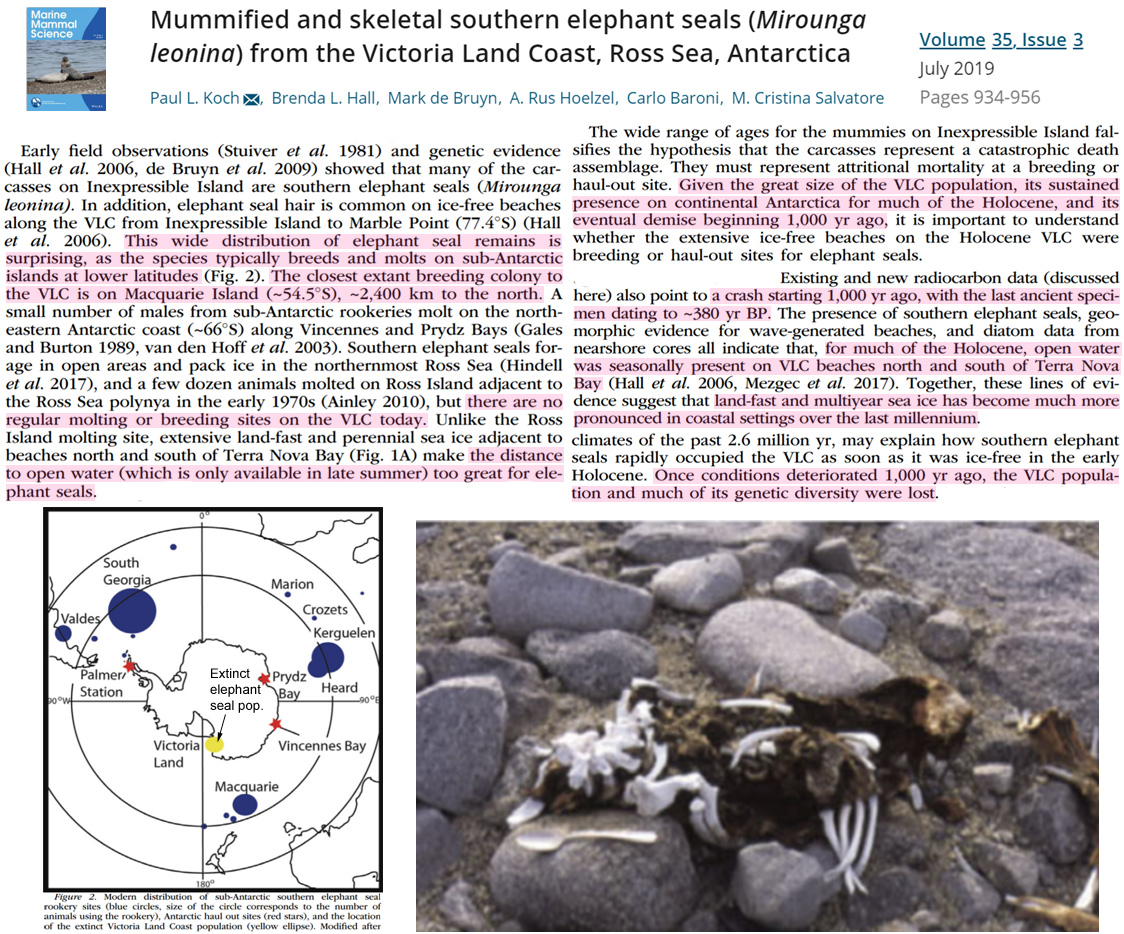